

How To Create Colored Maps In R
view raw Rmd
EDIT: Post-obit a proposition Adriano Fantini and lawmaking from Andy Due south, we replaced rworlmap past rnaturalearth.
This tutorial is the first part in a series of 3:
- General concepts illustrated with the globe Map (this document)
- Adding additional layers: an example with points and polygons
- Positioning and layout for complex maps
In this part, we will cover the fundamentals of mapping using ggplot2 associated to sf, and presents the basics elements and parameters nosotros tin play with to prepare a map.
Maps are used in a diversity of fields to express data in an appealing and interpretive way. Information tin exist expressed into simplified patterns, and this data interpretation is generally lost if the data is just seen through a spread sail. Maps can add together vital context past incorporating many variables into an easy to read and applicative context. Maps are also very of import in the data world because they can speedily permit the public to gain improve insight so that they can stay informed. It's critical to have maps be constructive, which ways creating maps that can exist hands understood past a given audience. For instance, maps that need to be understood past children would be very unlike from maps intended to be shown to geographers.
Knowing what elements are required to enhance your data is key into making effective maps. Basic elements of a map that should be considered are polygon, points, lines, and text. Polygons, on a map, are closed shapes such as state borders. Lines are considered to exist linear shapes that are not filled with any attribute, such equally highways, streams, or roads. Finally, points are used to specify specific positions, such equally urban center or landmark locations. With that in listen, one need to think about what elements are required in the map to actually make an bear upon, and convey the information for the intended audition. Layout and formatting are the second disquisitional aspect to raise data visually. The organization of these map elements and how they will be drawn can be adjusted to make a maximum impact.
A solution using R and its ecosystem of packages
Current solutions for creating maps ordinarily involves GIS software, such equally ArcGIS, QGIS, eSpatial, etc., which allow to visually prepare a map, in the same approach as i would set up a affiche or a certificate layout. On the other hand, R, a complimentary and open-source software evolution environment (IDE) that is used for calculating statistical data and graphic in a programmable language, has developed advanced spatial capabilities over the years, and can be used to describe maps programmatically.
R is a powerful and flexible tool. R can be used from calculating data sets to creating graphs and maps with the same data set up. R is too gratis, which makes it easily accessible to anyone. Some other advantages of using R is that it has an interactive language, data structures, graphics availability, a developed community, and the advantage of adding more functionalities through an unabridged ecosystem of packages. R is a scriptable language that allows the user to write out a code in which it will execute the commands specified.
Using R to create maps brings these benefits to mapping. Elements of a map can be added or removed with ease — R code tin exist tweaked to brand major enhancements with a stroke of a fundamental. It is also easy to reproduce the same maps for different data sets. It is of import to exist able to script the elements of a map, and then that it tin can be re-used and interpreted by any user. In essence, comparing typical GIS software and R for cartoon maps is similar to comparing give-and-take processing software (due east.g. Microsoft Office or LibreOffice) and a programmatic typesetting system such as LaTeX, in that typical GIS software implement a WYSIWIG approach ("What You See Is What You lot Get"), while R implements a WYSIWYM approach ("What You Run into Is What Y'all Mean").
The package ggplot2 implements the grammer of graphics in R, every bit a style to create code that brand sense to the user: The grammar of graphics is a term used to breaks upwardly graphs into semantic components, such as geometries and layers. Practically speaking, it allows (and forces!) the user to focus on graph elements at a college level of abstraction, and how the information must be structured to attain the expected outcome. While ggplot2 is becoming the de facto standard for R graphs, it does not handle spatial data specifically. The current state-of-the-art of spatial objects in R relies on Spatial classes defined in the bundle sp, but the new packet sf has recently implemented the "elementary feature" standard, and is steadily taking over sp. Recently, the bundle ggplot2 has allowed the utilise of uncomplicated features from the package sf as layers in a graph1. The combination of ggplot2 and sf therefore enables to programmatically create maps, using the grammar of graphics, just as informative or visually appealing as traditional GIS software.
Getting started
Many R packages are bachelor from CRAN, the Comprehensive R Archive Network, which is the main repository of R packages. The full list of packages necessary for this serial of tutorials tin can exist installed with:
install.packages(c("cowplot", "googleway", "ggplot2", "ggrepel", "ggspatial", "libwgeom", "sf", "rnaturalearth", "rnaturalearthdata") Nosotros start by loading the bones packages necessary for all maps, i.e. ggplot2 and sf. We too propose to use the classic night-on-light theme for ggplot2 (theme_bw), which is appropriate for maps:
library("ggplot2") theme_set(theme_bw()) library("sf") The package rnaturalearth provides a map of countries of the entire earth. Use ne_countries to pull country data and choose the calibration (rnaturalearthhires is necessary for calibration = "large"). The function can render sp classes (default) or directly sf classes, as divers in the argument returnclass:
library("rnaturalearth") library("rnaturalearthdata") world <- ne_countries(scale = "medium", returnclass = "sf") class(world) ## [one] "sf" ## [1] "data.frame" Full general concepts illustrated with the earth map
Data and basic plot (ggplot and geom_sf)
Start, allow us kickoff with creating a base of operations map of the world using ggplot2. This base map will then exist extended with dissimilar map elements, as well as zoomed in to an area of interest. We can check that the world map was properly retrieved and converted into an sf object, and plot it with ggplot2:
ggplot(information = world) + geom_sf() 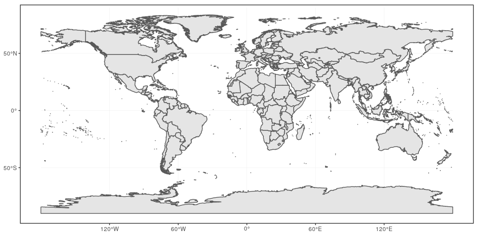
This telephone call nicely introduces the construction of a ggplot call: The first office ggplot(data = world) initiates the ggplot graph, and indicates that the main data is stored in the world object. The line ends upwardly with a + sign, which indicates that the telephone call is non complete yet, and each subsequent line correspond to some other layer or calibration. In this example, nosotros use the geom_sf part, which simply adds a geometry stored in a sf object. By default, all geometry functions utilize the main data defined in ggplot(), but we will see later how to provide additional information.
Note that layers are added one at a time in a ggplot call, so the order of each layer is very important. All information will have to exist in an sf format to exist used by ggplot2; data in other formats (e.m. classes from sp) volition be manually converted to sf classes if necessary.
Title, subtitle, and centrality labels (ggtitle, xlab, ylab)
A title and a subtitle can be added to the map using the function ggtitle, passing any valid character cord (e.g. with quotation marks) as arguments. Axis names are absent by default on a map, merely can be changed to something more suitable (e.k. "Longitude" and "Latitude"), depending on the map:
ggplot(data = world) + geom_sf() + xlab("Longitude") + ylab("Latitude") + ggtitle("Earth map", subtitle = paste0("(", length(unique(earth$Proper name)), " countries)")) 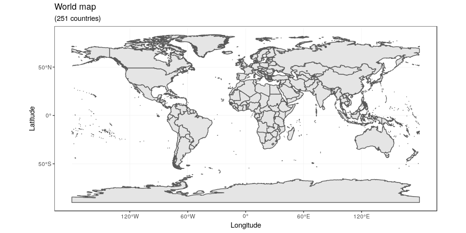
Map color (geom_sf)
In many ways, sf geometries are no different than regular geometries, and can be displayed with the same level of command on their attributes. Here is an example with the polygons of the countries filled with a dark-green color (argument fill), using black for the outline of the countries (argument colour):
ggplot(data = world) + geom_sf(color = "black", fill = "lightgreen") 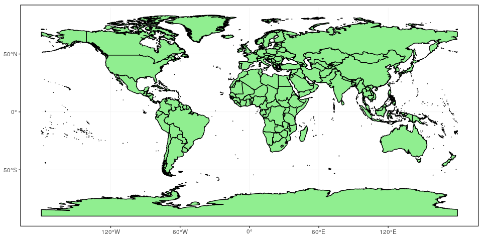
The package ggplot2 allows the apply of more circuitous colour schemes, such as a gradient on 1 variable of the data. Here is another case that shows the population of each state. In this instance, we utilize the "viridis" colorblind-friendly palette for the colour gradient (with selection = "plasma" for the plasma variant), using the foursquare root of the population (which is stored in the variable POP_EST of the world object):
ggplot(data = world) + geom_sf(aes(fill = pop_est)) + scale_fill_viridis_c(selection = "plasma", trans = "sqrt") 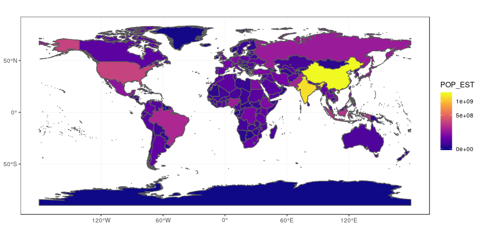
Projection and extent (coord_sf)
The function coord_sf allows to deal with the coordinate system, which includes both projection and extent of the map. Past default, the map will utilize the coordinate arrangement of the first layer that defines i (i.e. scanned in the guild provided), or if none, fall back on WGS84 (breadth/longitude, the reference system used in GPS). Using the argument crs, it is possible to override this setting, and project on the wing to any project. This can be achieved using whatever valid PROJ4 cord (here, the European-axial ETRS89 Lambert Azimuthal Equal-Area project):
ggplot(information = world) + geom_sf() + coord_sf(crs = "+proj=laea +lat_0=52 +lon_0=10 +x_0=4321000 +y_0=3210000 +ellps=GRS80 +units=m +no_defs ") 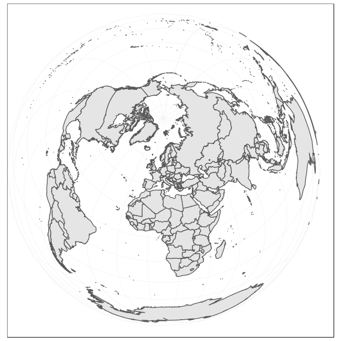
Spatial Reference Organization Identifier (SRID) or an European Petroleum Survey Grouping (EPSG) lawmaking are available for the projection of interest, they tin can be used directly instead of the full PROJ4 string. The 2 following calls are equivalent for the ETRS89 Lambert Azimuthal Equal-Surface area projection, which is EPSG code 3035:
ggplot(data = world) + geom_sf() + coord_sf(crs = "+init=epsg:3035") ggplot(data = world) + geom_sf() + coord_sf(crs = st_crs(3035)) The extent of the map tin can also be fix in coord_sf, in practice allowing to "zoom" in the area of involvement, provided by limits on the x-axis (xlim), and on the y-centrality (ylim). Note that the limits are automatically expanded past a fraction to ensure that data and axes don't overlap; it can too be turned off to exactly match the limits provided with aggrandize = FALSE:
ggplot(information = world) + geom_sf() + coord_sf(xlim = c(-102.15, -74.12), ylim = c(7.65, 33.97), expand = FALSE) 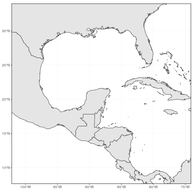
Scale bar and North arrow (packet ggspatial)
Several packages are available to create a scale bar on a map (e.one thousand. prettymapr, vcd, ggsn, or legendMap). We innovate here the packet ggspatial, which provides easy-to-use functions…
scale_bar that allows to add simultaneously the north symbol and a scale bar into the ggplot map. Five arguments need to be set manually: lon, lat, distance_lon, distance_lat, and distance_legend. The location of the scale bar has to be specified in longitude/latitude in the lon and lat arguments. The shaded distance within the scale bar is controlled past the distance_lon argument. while its width is adamant by distance_lat. Additionally, information technology is possible to change the font size for the fable of the calibration bar (statement legend_size, which defaults to iii). The N arrow behind the "N" north symbol can also be adapted for its length (arrow_length), its distance to the scale (arrow_distance), or the size the N northward symbol itself (arrow_north_size, which defaults to vi). Annotation that all distances (distance_lon, distance_lat, distance_legend, arrow_length, arrow_distance) are gear up to "km" by default in distance_unit; they tin also be set up to nautical miles with "nm", or miles with "mi".
library("ggspatial") ggplot(data = world) + geom_sf() + annotation_scale(location = "bl", width_hint = 0.5) + annotation_north_arrow(location = "bl", which_north = "true", pad_x = unit(0.75, "in"), pad_y = unit(0.v, "in"), style = north_arrow_fancy_orienteering) + coord_sf(xlim = c(-102.fifteen, -74.12), ylim = c(seven.65, 33.97)) ## Scale on map varies past more than than 10%, calibration bar may be inaccurate 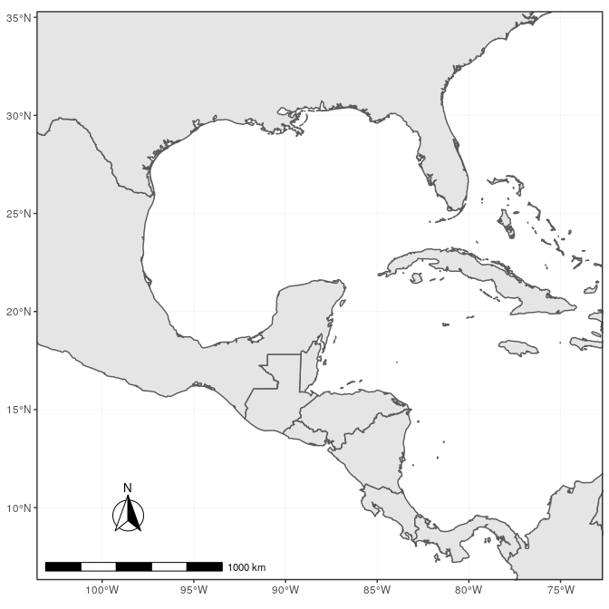
Note the alarm of the inaccurate scale bar: since the map utilise unprojected data in longitude/latitude (WGS84) on an equidistant cylindrical projection (all meridians beingness parallel), length in (kilo)meters on the map directly depends mathematically on the degree of breadth. Plots of small regions or projected information will frequently let for more than authentic scale confined.
State names and other names (geom_text and annotate)
The globe data set already contains country names and the coordinates of the centroid of each country (amidst more information). We tin employ this data to plot country names, using world as a regular data.frame in ggplot2. The function geom_text can be used to add together a layer of text to a map using geographic coordinates. The function requires the information needed to enter the country names, which is the same data every bit the world map. Once more, we take a very flexible control to adjust the text at will on many aspects:
- The size (argument
size); - The alignment, which is centered by default on the coordinates provided. The text can be adjusted horizontally or vertically using the arguments
hjustandvjust, which tin either be a number between 0 (right/lesser) and ane (top/left) or a character ("left", "center", "correct", "bottom", "center", "acme"). The text can besides be offset horizontally or vertically with the argumentnudge_xandnudge_y; - The font of the text, for case its colour (argument
color) or the type of font (fontface); - The overlap of labels, using the statement
check_overlap, which removes overlapping text. Alternatively, when there is a lot of overlapping labels, the packageggrepelprovides ageom_text_repelfunction that moves label effectually so that they practice not overlap. - For the text labels, nosotros are defining the centroid of the counties with
st_centroid, from the packagesf. Then we combined the coordinates with the centroid, in thegeometryof the spatial data frame. The packagesfis necessary for the controlst_centroid.
Additionally, the annotate function can exist used to add together a single character string at a specific location, as demonstrated here to add together the Gulf of Mexico:
library("sf") world_points<- st_centroid(world) world_points <- cbind(world, st_coordinates(st_centroid(globe$geometry))) ggplot(information = earth) + geom_sf() + geom_text(data= world_points,aes(10=10, y=Y, label=name), colour = "darkblue", fontface = "bold", check_overlap = FALSE) + annotate(geom = "text", x = -90, y = 26, characterization = "Gulf of United mexican states", fontface = "italic", color = "grey22", size = vi) + coord_sf(xlim = c(-102.15, -74.12), ylim = c(7.65, 33.97), expand = False) 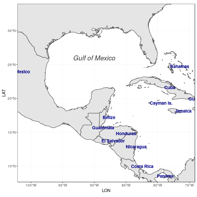
Final map
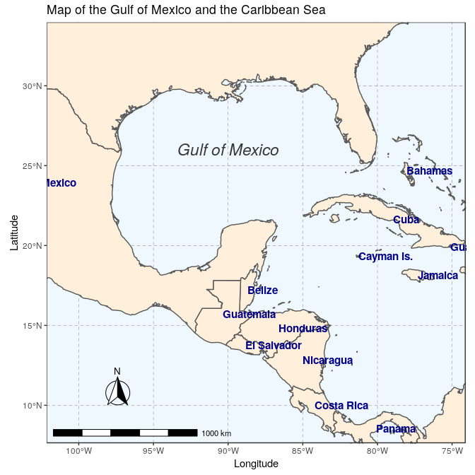
Now to make the final touches, the theme of the map tin can exist edited to make it more than appealing. We suggested the use of theme_bw for a standard theme, only there are many other themes that tin be selected from (meet for case ?ggtheme in ggplot2, or the package ggthemes which provide several useful themes). Moreover, specific theme elements can be tweaked to become to the concluding upshot:
- Position of the fable: Although not used in this example, the argument
legend.positionallows to automatically place the legend at a specific location (e.yard."topright","bottomleft", etc.); - Grid lines (graticules) on the map: by using
console.grid.majorandpanel.grid.minor, grid lines can be adjusted. Here nosotros set up them to a gray color and dashed line type to clearly distinguish them from country borders lines; - Map background: the statement
panel.backgroundcan be used to color the background, which is the ocean essentially, with a low-cal bluish; -
Many more elements of a theme can be adapted, which would exist besides long to comprehend hither. We refer the reader to the documentation for the function
theme.ggplot(data = globe) + geom_sf(fill= "antiquewhite") + geom_text(data= world_points,aes(10=X, y=Y, label=name), color = "darkblue", fontface = "bold", check_overlap = Faux) + comment(geom = "text", x = -90, y = 26, label = "Gulf of Mexico", fontface = "italic", color = "grey22", size = 6) + annotation_scale(location = "bl", width_hint = 0.5) + annotation_north_arrow(location = "bl", which_north = "true", pad_x = unit of measurement(0.75, "in"), pad_y = unit(0.v, "in"), style = north_arrow_fancy_orienteering) + coord_sf(xlim = c(-102.15, -74.12), ylim = c(vii.65, 33.97), aggrandize = FALSE) + xlab("Longitude") + ylab("Latitude") + ggtitle("Map of the Gulf of United mexican states and the Caribbean Ocean") + theme(panel.grid.major = element_line(color = greyness(.5), linetype = "dashed", size = 0.five), panel.background = element_rect(make full = "aliceblue"))
Saving the map with ggsave
The last map at present ready, information technology is very easy to save it using ggsave. This function allows a graphic (typically the last plot displayed) to be saved in a variety of formats, including the most common PNG (raster bitmap) and PDF (vector graphics), with control over the size and resolution of the event. For instance hither, we save a PDF version of the map, which keeps the best quality, and a PNG version of it for web purposes:
ggsave("map.pdf") ggsave("map_web.png", width = half-dozen, height = 6, dpi = "screen") 
How To Create Colored Maps In R,
Source: https://r-spatial.org/r/2018/10/25/ggplot2-sf.html
Posted by: bickerstaffwainewhim.blogspot.com
0 Response to "How To Create Colored Maps In R"
Post a Comment